Merry's Dev. Blog

개요

• 이번부터 쓰는 글은 Tensorflow-models 중 hand-pose-detection 을 자사 제품 내에서 구현한 후, 그와 관련된 AI 이론을 정리한 내용임
• 이번 글 출처: 학부 강의 내용, 필기, 구글링, 필요하다면 이하에서 출처 명시했음

1. 서

의미

• 2개 이상의 hidden layer를 가지고 있는 Neural Network 모형
  → 즉 2개 이상 = deep 하다 라고 생각하여 Deep Neural Network (이하 DNN) 라고 이름 붙여짐 
• 그림
  • 출처: https://www.i2tutorials.com/explain-deep-neural-network-and-shallow-neural-networks/#google_vignette

• hidden layer가 2개 이상인 이유
  : 풀고자 하는 문제를 세부 문제로 나누고, 그 문제를 다시 세세부 문제로 나누기 때문
  (ex) 사람의 얼굴인가 → 오른쪽 위에 눈이 있는가 → 위에 눈썹이 있는가, 가운데에 눈동자가 있는가, 아래에 속눈썹이 있는가

Support vector machine과의 비교

• SVM (Support Vector Machine)
  • 머신러닝 분야 중 하나로 ①패턴 인식, 자료 분석을 위한 지도 학습 모델 분류와 ②회귀 분석을 위해 사용됨
  • SVM의 패턴 인식 순서
    1. 2개 카테고리 중 어느 하나에 속한 데이터 집합이 주어졌을 때,
    2. 그것을 바탕으로 비확률적 이진 선형분류모델을 만듦. 이 모델은 새로운 데이터가 둘 중 어떤 카테고리에 속하는지 판단함
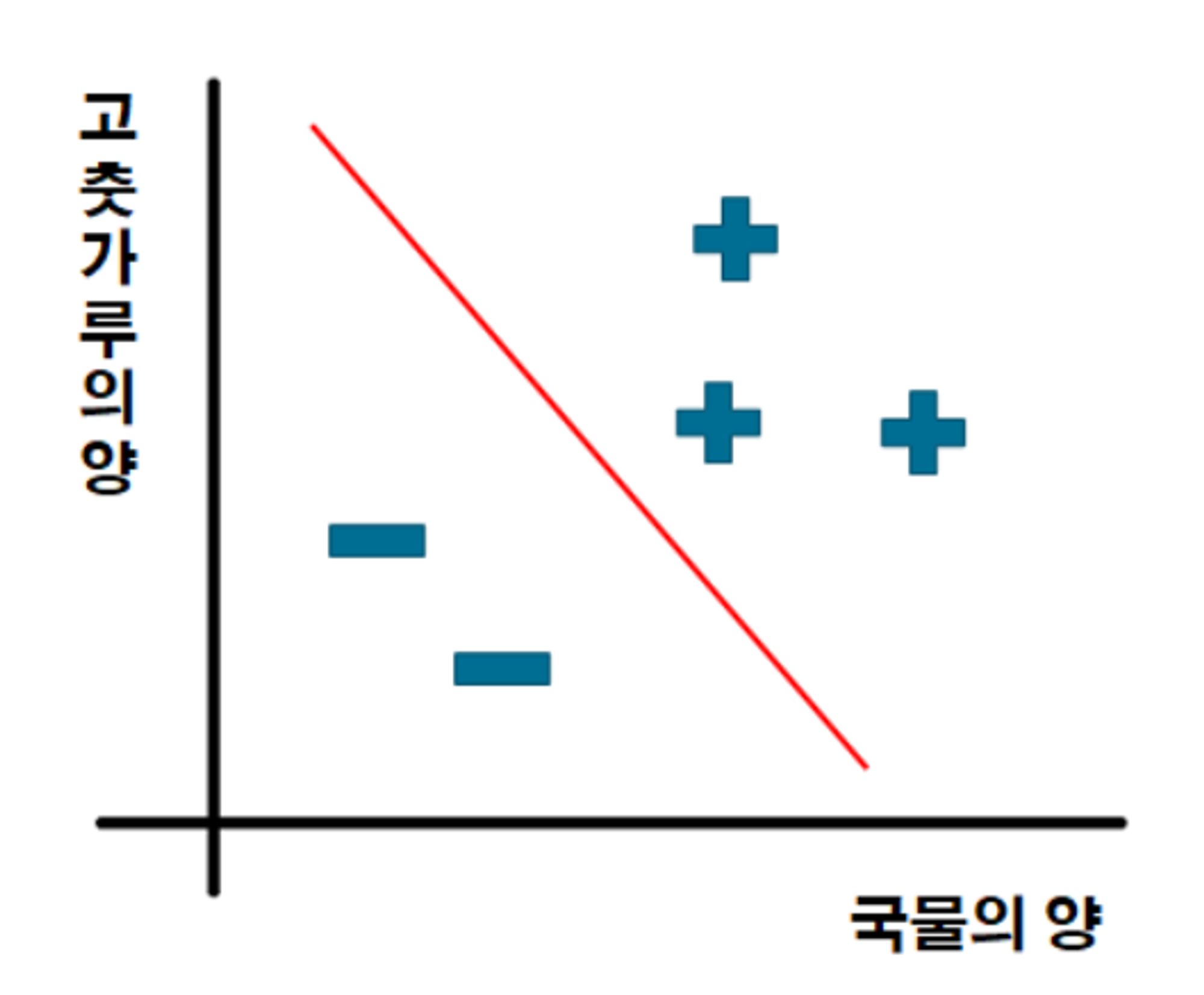
    3. 해당 모델은 데이터가 분포된 공간에서 선을 그어 경계를 표현함. 그리고 SVM 알고리즘은 그 중 가장 큰 폭을 가진 경계를 찾음
  • 예시 : 이진 분류를 한다면 밑 사진처럼 직선(linear decision boundary)을 그어 구분하는 것
    -> 출처: https://sanghyu.tistory.com/7

• 비교

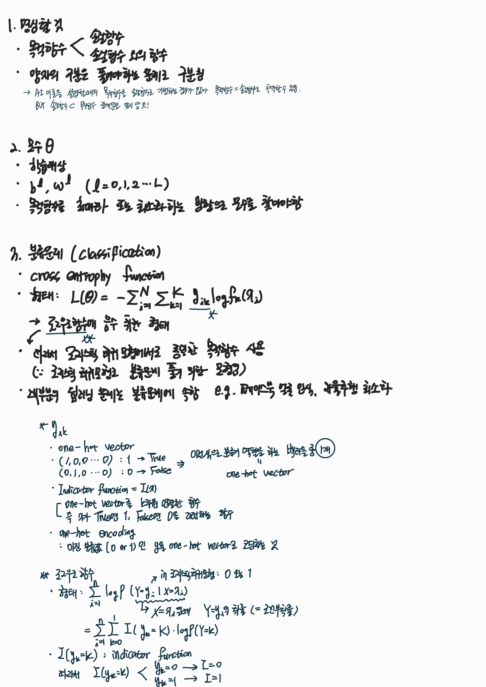
2. 모형 

모수의 학습 방법 
: 목적 함수 및 함수 구조를 기반으로 최적화 알고리즘 설명

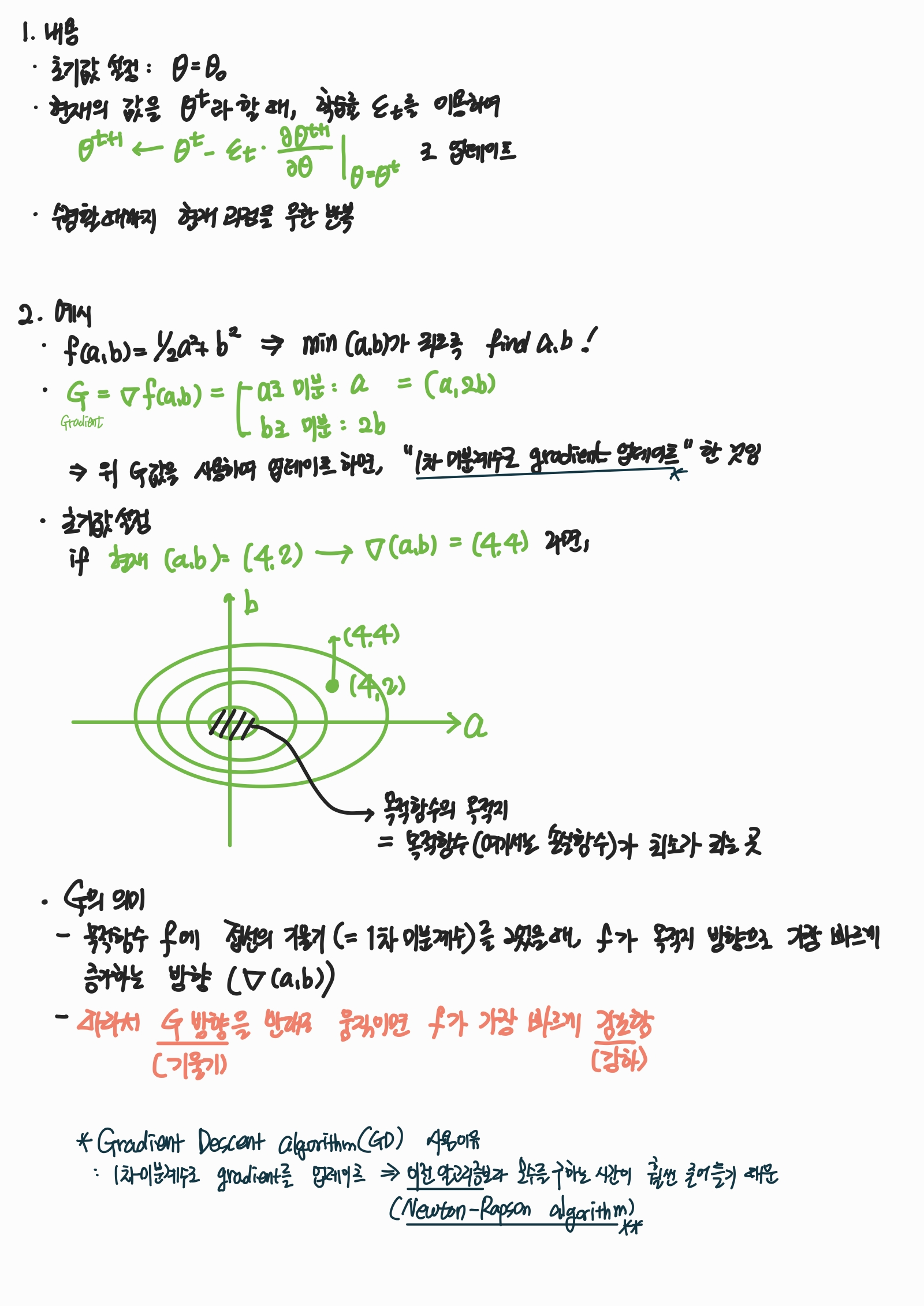
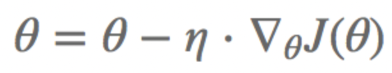
1. 기울기 강화 알고리즘 (Gradient Descent algorithm; GD)

• 특정 목적 함수 L(θ)를 최소화하는 θ을 한 번에 찾기 힘든 경우에 사용하는 대표적인 반복 알고리즘.
• 목적 함수 의미

• GD의 아이디어

• 구체적인 알고리즘 내용

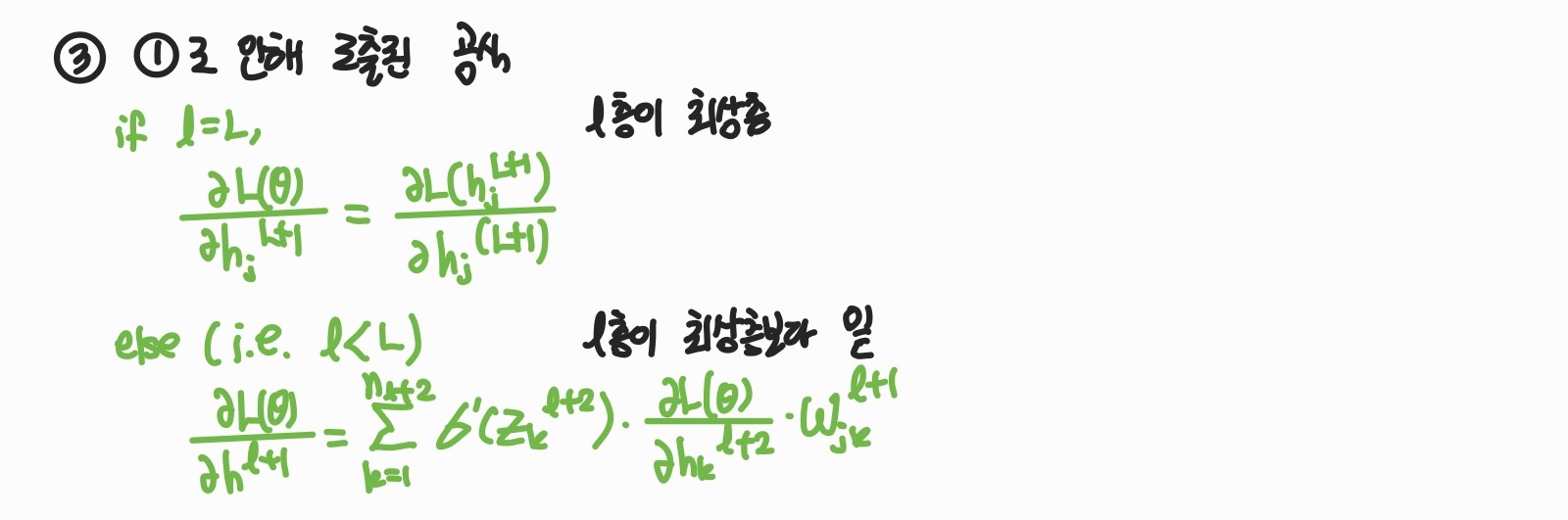
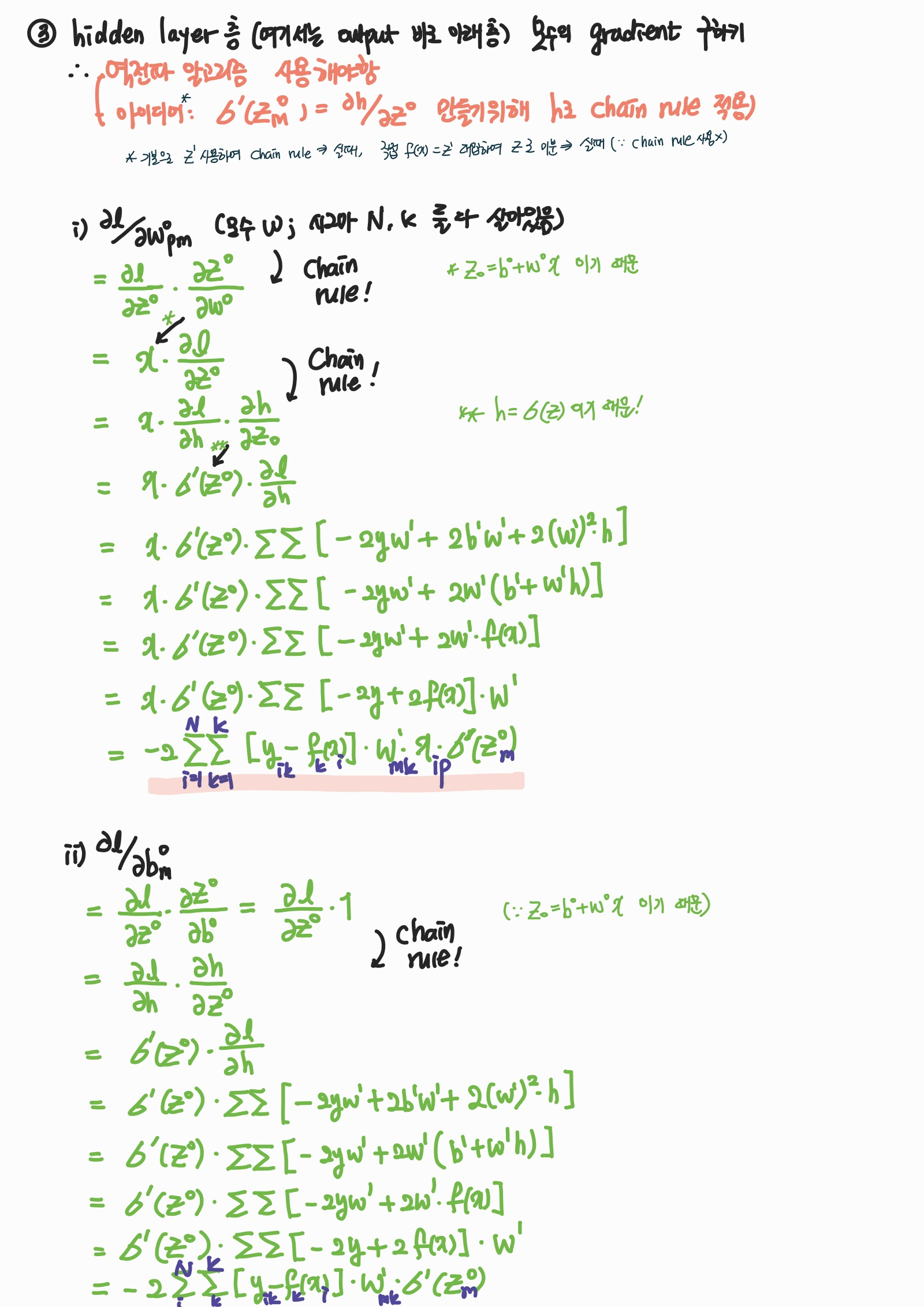
   2. 역전파 알고리즘 (Back propagation algorithm)

• 의미
  • 미분값이 위에서 아래로 계산되어짐 (Back propagation)
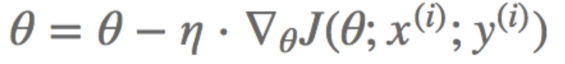
  • DNN 모수들의 (b, w) gradient를 구하는 알고리즘
  • 목적 함수 L(θ)을 최소화하기 위해 gradient descent algorithm을 사용한 결과,
    NN의 특수한 형태 때문에 ∂L(θ) / ∂θ(l+1)의 계산에 필요한 값을 알고 있으면, ∂L(θ) / ∂θ(l)가 자동적으로 계산됨.
    (여기서 θ(l)은 l층에서의 모수)
• 수식으로 의미 이해
  • 실제 숫자를 넣어 gradient를 계산한 레퍼런스
    https://wikidocs.net/37406 https://jaejunyoo.blogspot.com/2017/01/backpropagation.html
  • 나의 이해

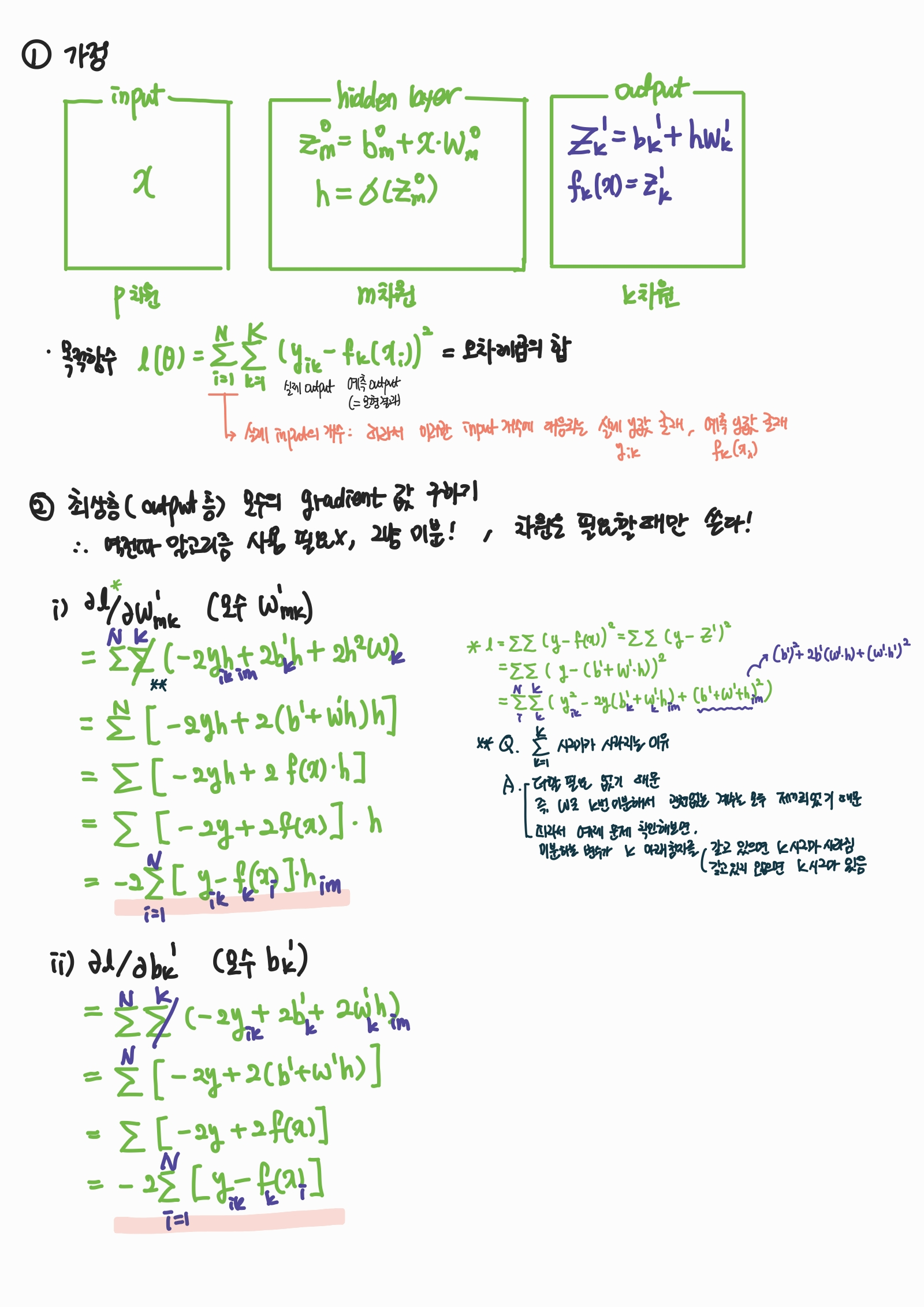
• 예제
  • 문제: Calculate gradient 에 있는 수식을 도출하는게 목적!
   

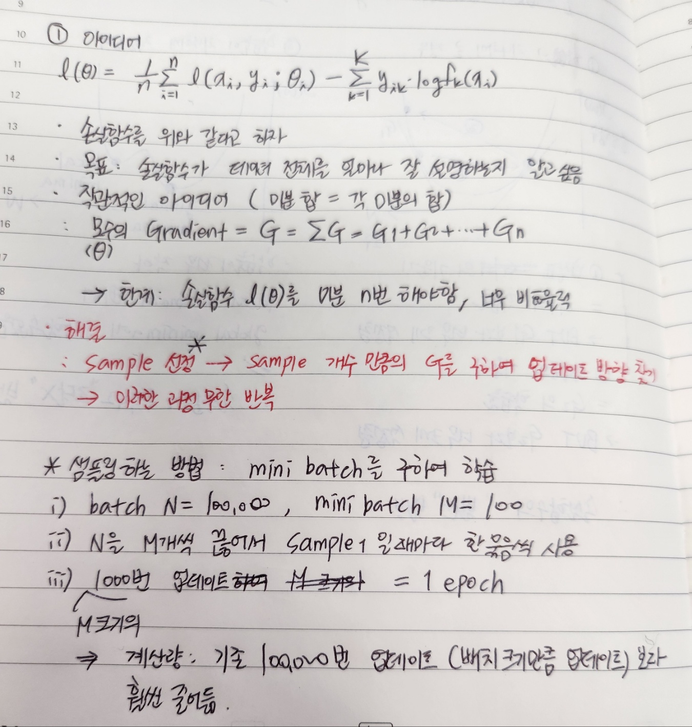
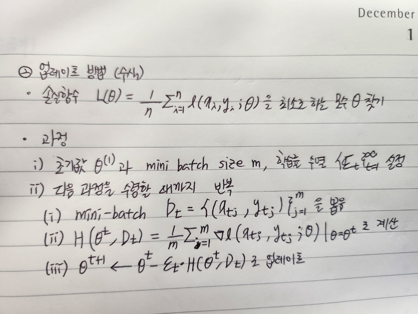
  3. Stochastic gradient descent method (SGD)

• 기본 용어 정리
  • Batch : 학습 데이터 전체
  • Mini-batch : 학습 데이터의 일부, 즉 batch에서 sampling 한 것
  • Epoch : 반복적인 학습 알고리즘을 사용할 때 모든 학습 데이터를 한 번 씩 사용하는 것을 의미
    (ex: 10000개의 학습 데이터가 존재하고, 매번 50개의 데이터(i.e. 50개의 mini-batch)를 이용하여 모수를 학습할 때, 이 알고리즘을 200번을 반복하면 1 epoch, 400번을 반복하면 2 epochs라고 함.)
    → 즉 1 에폭당 학습 데이터 10000개를 한 바퀴 도는 느낌
• 의미
  • Stochastic gredient descent algorithm을 사용한 method
  • 아이디어 및 업데이트 방법

• 장점
  • 계산량↓: 업데이트 할 때 모든 batch를 사용할 때보다 적은 계산을 필요로 함
  • 정확성↑: 수렴성이 이론적으로 보장 (Bottou, 1998 and Murata, 1998)
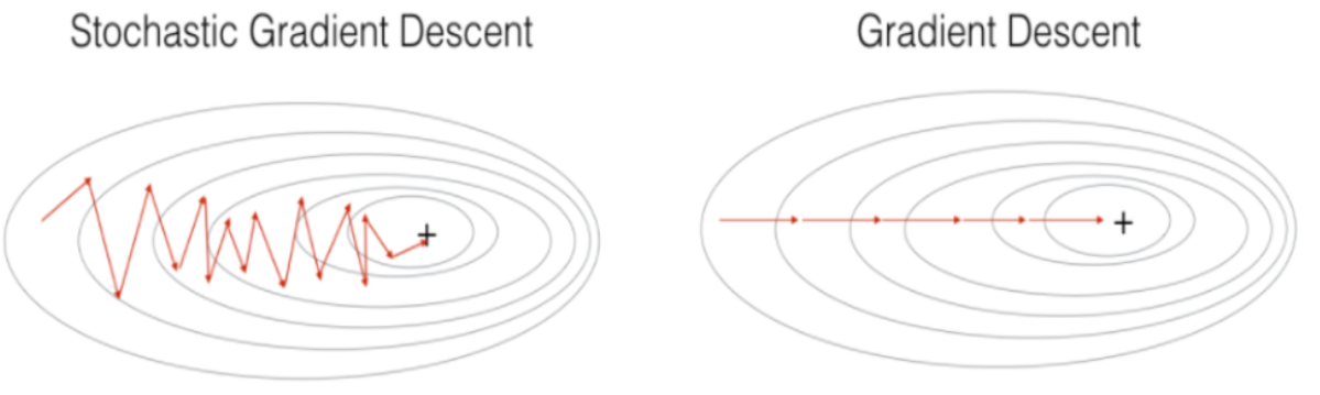
• gredient descent algorithm과의 차이
  • 핵심
    • Gradient Descent (GD): mini batch 사용하지 않고 학습 → 에폭이 1인 SGD 느낌
    • Stochastic Gradient Descent (SGD): mini batch 를 샘플링하여 학습 → 파생적으로 에폭의 개념 나오게 됨
  • 수식
        - GD

                  - SGD 

•     그림
               

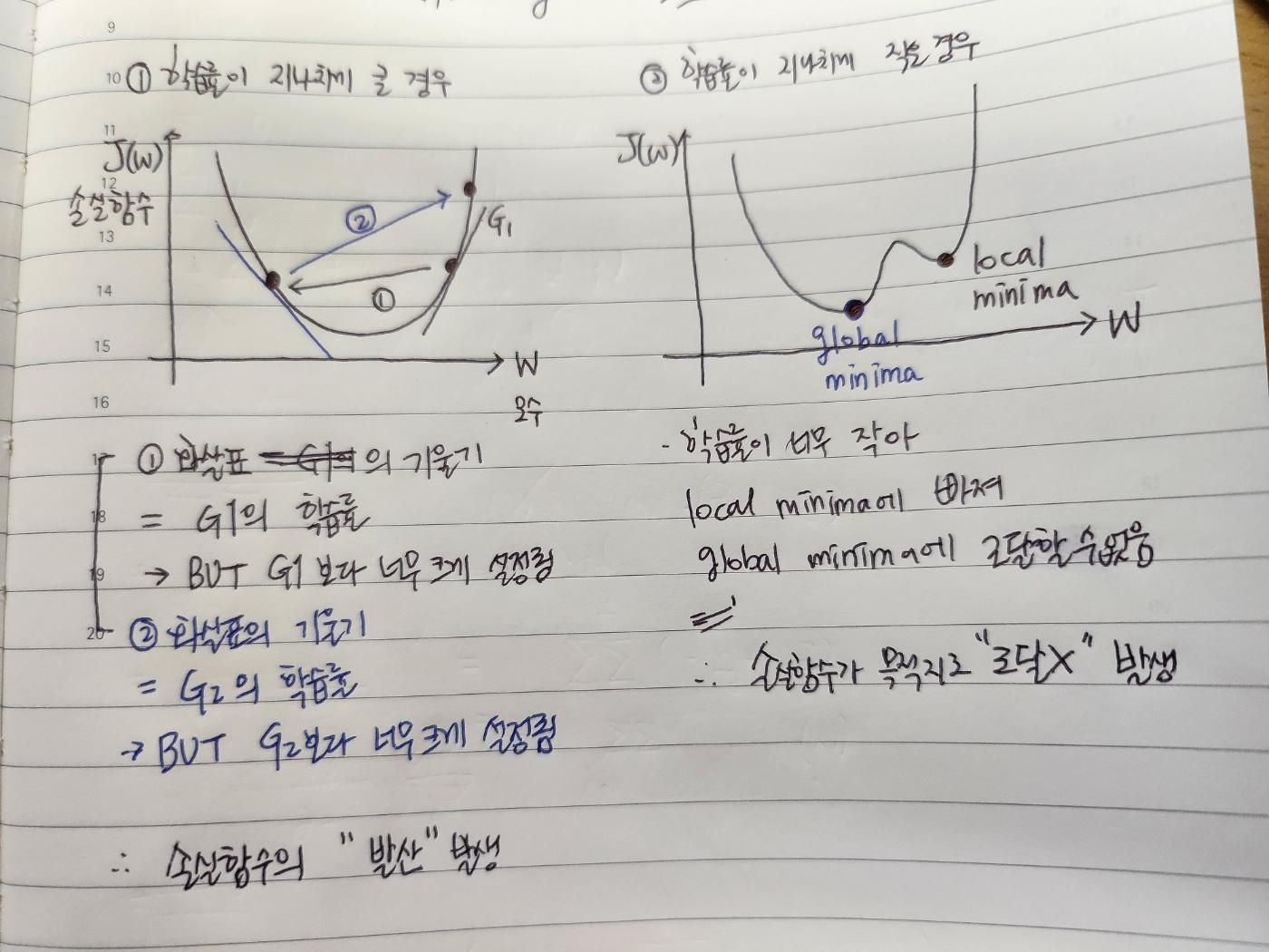
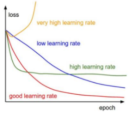
2. 학습률 (learning rate) 의 선택

의미

• 목적 함수의 최댓값 또는 최솟값을 향해 이동하면서 각 반복에서 단계 크기를 결정하는 스칼라
• 학습률은 머신러닝 및 통계학에서 사용되는 용어
• 최적화 알고리즘의 조정 매개변수
• εt∶ t 시점의 학습률

특징

• 학습률이 지나치게 크거나 작으면 좋은 추정값을 얻을 수 없음. 목적 함수가 목적지로 발산 or 도달하지 못하기 때문임
• 따라서 학습이 진행될수록 비교적 큰 학습률 → t가 증가함에 따라 학습률을 줄여나가는 것이 바람직함
• 이론적으로는 εt ∝1/t이면 (비례하다면), 역전파 알고리즘을 사용하였을 때 손실 함수가 국소적인 최소값으로 수렴한다는 사실이 알려져 있음. (Bottou et al., 2018)

3. 한계

Vanishing gradients problem

• 모수에 대한 gradient 값이 아래층으로 내려갈수록 작아지는 현상.
  = 즉, hidden layer 쌓을수록 추정 값 정확도↓ (=성능↓)
• 그 결과 아래층의 모수가 초기 값과 크게 다르지 않은 값을 가진 채 학습이 종료.
  = 즉, 안 좋은 모수를 갖는 추정 값으로 수렴함
• 따라서, 때때로 DNN이 NN 보다 성능이 나쁜 경우 발생함
• 원인: 역전파 알고리즘이 좋지 않은 추정값을 제공 (bad local minima).

Running time

• 일반적으로 DNN은 1개의 hidden layer를 가지는 NN보다 더 많은 수의 모수를 필요로 함
• 더 많은 수의 모수를 추정하기 위해 보다 더 많은 시간 소요됨

보완책: 사전 학습 (Pre-training)

• 2006년 G.E.Hinton 교수가 처음으로 제안: Hinton and Salakhutdinov (2006), Hinton et al (2006)
• 입력 변수만 사용하여 모수를 추정하는 기법 (Pre-training) → 추청된 모수를 학습 시 초기값으로 사용 (Training)
  → 이 방법이 이전 방법과 다른 이유: 기존 training은 입력 값, 출력 값을 모두 이용하여 학습
• 효과: 역전파 알고리즘의 한계 해결
  • 결과가 해의 초기값에 의존
    = 즉 아래층에 있는 모수들은 초기 값과 크게 다르지 않음
  • 그러나 좋은 해의 초기값을 찾기 어려움
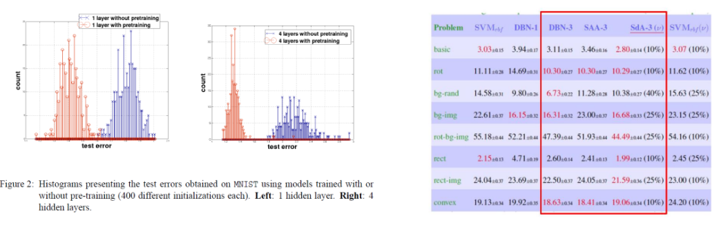
• 예시: Erhan et al., 2010 and Larochelle et al., 2007
  • 왼쪽 그래프: hidden layer 1층, 오른쪽 그래프: hidden layer 4층
  • hidden layer의 개수가 늘어날수록 pre-training 한 layer의 효과가 더 커짐
    = 즉 데이터의 test error 가 작아짐

4. Advanced of deep learning

하드웨어의 발전: GPU의 사용

• 딥러닝에서 필요한 계산들을 대부분 병렬처리 가능
• 따라서 CPU로 계산할 때보다 훨씬 빠른 계산 가능
  + 훨씬 많은 hidden layer와 모수들을 가지는 복잡한 모형 설계하여 활용 가능

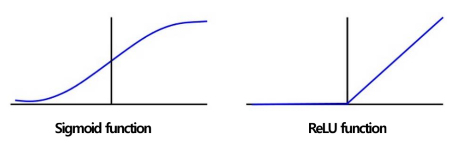
새로운 활성 함수의 개발: ReLU (Rectified Linear Units; Nair and Hinton (2010))

• 우수성
  • 기존의 활성함수 (예: sigmoid or tanh)는 그 특성상 모수를 추정하는데 어려움
    (어려움: vanishing gradient)
  • Piece-wise 선형 함수를 활성함수로 사용
    → vanishing gradient 문제 해결, 속도 향상, 사전 학습 불필요해짐
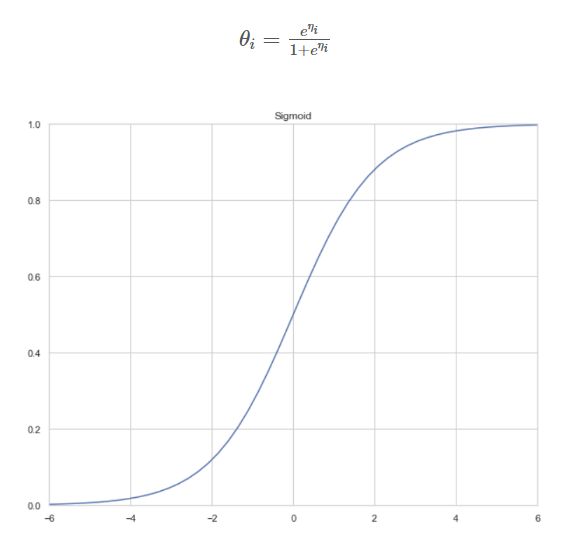
• sigmoid 함수와 비교

• 이후에 ReLU를 응용하여 LeakyReLU (Mass et al., 2013), PReLU (He et al., 2015), ELU (Clevert et al., 2015) 등 많은 활성 함수가 제안됨.

Regularization method 개발

1. Drop out
   • 매번 역전파를 할 때마다 노드의 절반을 끄고 (=drop out) 학습
     → 최종 결과를 낼 떄에는 각 층 결과값에 1/2를 곱하는 방법
   • 효과: 노드 간 상관관계↓, 독립성↑
   • 원인: fully connected neural network을 학습할 때, 같은 층의 노드간에 높은 상관관계 발생
     → 입력값이 조금만 바뀌어도 모든 네트워크에 큰 변화가 생길 수 있음
2. Batch normalization
   • 매번 mini batch를 이용하여 학습할 떄마다 노드들을 정규화함
   • 효과: 적은 에폭 학습을 하여도 기존보다 좋은 성능 (ex. 보다 높은 accuracy)를 얻을 수 있게 됨
   • 원인: 은닉 노드 각각의 분포 및 scale이 상이 → 성능이 좋지 않음
3. Data augmentation (데이터 증강)
   • Random crop, RGB perturbation, image reflection 등으로 학습 데이터를 대량 확보하는 것
   • 심지어 Sequential data에서도 data의 순서를 바꾸어 학습 데이터를 늘림.
   • 효과: 모델이 정확한 예측을 하기 위한 재료가 다수 확보됨
     → 보다 정확한 예측 가능
   • 원인: 학습 대상 데이터의 양이 지나치게 적은 경우, 학습이 제대로 되기 어려움
4. Residual learning architecture (잔차 학습 아키텍처)
   • Networks에서 이웃하지 않은 layer 사이에도 connection을 추가
   • 효과: Vanishing problem 해결

5. Advanced of learning algorithms

SGD 방법의 단점

1. 학습률 εk의 scale에 따라 성능이 크게 좌우됨.
   = 손실 함수들마다 좋은 성능을 보장하는 학습률 scale이 달라 선택이 어려움

  2. 이전 gradient 정보들은 무시하고 현 시점의 gradient만을 사용하여 업데이트
      → 수렴 속도가 느릴 수 있음

  3. 시점 k에서 모든 gradient에 미리 정해 놓은 학습률 εk를 곱해주어 업데이트.
      → 손실함수가 특정 모수들의 방향에 대해서 민감하게 변할 경우에 수렴하지 않을 수 있음.
      → 안장점*에 빠질 가능성이 높음.

      * 안장점 (Saddle point)
      - 다변수 함수에서 특정한 형태의 극값.
        = 한 쪽 방향에서 보면 극댓값, 다른 쪽 방향에서 보면 극솟값
      - 예시 : 이차항이 마이너스인 이차함수
        -> 안장점 (이자 극댓값)에서 한 방향에서는 곡면이 상승, 다른 방향에서는 하강

        - 머신러닝에서의 안장점 
          > 신경망 모형(NN)을 학습시킬 때 최적화 알고리즘이 안장점에 도달한 경우,
            여기서 멈추지 않고 전역 최소점 (global minimum) 또는 국소 최소점 (local minimum) 에 도달할 수 있도록 설계해야함
            ( ∵ 최적화 알고리즘의 목표 = 목적함수(손실함수) 최소화)
          > 따라서 이것이 머신러닝 또는 딥러닝의 성능을 결정지음

SGD with momentum

• 현 시점의 gradient 업데이트 방향이 이전 시점의 gradient 정보에 영향을 받는 방법
  = 즉 현재 및 과거 시점의 gradient 크기에(g) 영향을 받아서 모수들(θ) 각각의 학습률이(ε) 결정됨
• Goodfellow, I., et al. (2016) Deep Learning : 모멘텀을 수식으로 증명

• 이는 “이전 gradient 정보들은 무시하고 현 시점의 gradient만을 사용하여 업데이트” 하는 SGD의 1번 단점을 보완한 것

adam

• ①accumulated squared gradient를 weighted average로 업데이트 함 (두 번째 빨간 박스)
  + ②현 시점의 gradient 업데이트 방향이 이전 시점의 gradient 정보에 영향을 받아 결정됨 (첫 번째 빨간 박스)
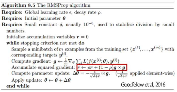
  = ①RMSProp* + ②momentum
  • RMSProp (Tieleman and Hinton, 2012)
    • AdaGrad*와는 다르게 accumulated squared gradient를 누적 합으로 업데이트 하지 않고, weighted average로 업데이트 함.
      = 즉 AdaGrad의 단점 보완
    • Goodfellow, I., et al. (2016) Deep Learning : RMSProp을 수식으로 증명
      : 빨간 박스 수식 = weighted average

               * AdaGrad
                 : 현재 및 과거 시점의 gradient의 크기에 영향을 받아서 (첫 번째 빨간 박스)
                → 모수들 각각의 학습률이 결정됨 ( i.e. adaptive learning rate) (두 번째 빨간 박스)

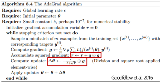
                  - 학습률이 미리 정해져 있지 않고, 합리적인 방법을 통해 결정된다는 점에서 SGD의 단점 중 1번, 3번이 해결됨 
                  - Goodfellow, I., et al. (2016) Deep Learning : AdaGrad을 수식으로 증명
                  - 한계 - 지속적인 업데이트가 진행됨에 따라 accumulated squared gradient의 r의 값이 너무 커져서 업데이트가 몇 차례 진행 되지 않아 모수의 추정값이 도중에 수렴해 버림

• Goodfellow, I., et al. (2016) Deep Learning : Adam을 수식으로 증명
  • 현재까지 나온 최적화 방법론들 중 일반적으로 빠르게 좋은 추정 값을 찾아 주는 알고리즘.
  • Convex loss function 뿐만 아니라 non-convex loss function (예: 딥러닝 모델에서의 손실함수) 에서 매우 좋은 성능을 제공.

개요

• 이번부터 시리즈로 쓰는 글은 Tensorflow-models 중 pose-detection 을 자사 제품 내에서 구현한 후, 그와 관련된 AI 이론을 정리한 내용임
• 이번 글 model card와 관련된 내용의 출처는 https://storage.googleapis.com/mediapipe-assets/Model%20Card%20BlazePose%20GHUM%203D.pdf

1. 모델 설명 | Used to

모델 설명

• 모델명: MediaPipe BlazePose GHUM 3D
• 구체적인 설명

Lite (3MB size), Full (6 MB size) and Heavy (26 MB size) models, to estimate the full 3D body pose of an individual in videos captured by a smartphone or web camera.
Optimized for on-device, real-time fitness applications: Lite model runs ~44 FPS on a CPU via XNNPack TFLite and ~49 FPS via TFLite GPU on a Pixel 3. Full model runs ~18 FPS on a CPU via XNNPack TFLite and ~40 FPS via TFLite GPU on a Pixel 3.
Heavy model runs ~4FPS on a CPU via XNNPack TFLite and ~19 FPS via TFLite GPU on a Pixel 3.

Used to

Applications
3D full body pose estimation for single-person videos on mobile, desktop and in browser.

Domain & Users
 - Augmented reality
 - 3D Pose and gesture recognition
 - Fitness and repetition counting
 - 3D pose measurements (angles / distances)

Out-of-scope applications
Multiple people in an image.
 - People too far away from the camera (e.g. further than 14 feet/4 meters)
 - Head is not visible Applications requiring metric accurate depth
 - Any form of surveillance or identity recognition is explicitly out of scope and not enabled by this technology

2. Model type 및 Model architecture

모델 카드 인용

Convolutional Neural Network: MobileNetV2-like with customized blocks for real-time performance.

Model type: CNN

Model architecture : MobileNetV2

3. input, output

Inputs
Regions in the video frames where a person has been detected.
Represented as a 256x256x3 array with aligned human full body part, centered by mid-hip in vertical body pose and rotation distortion of (-10, 10) . Channels order: RGB with values in [0.0, 1.0].

Output(s)
33x5 array corresponding to (x, y, z, visibility, presence).
 - X, Y coordinates are local to the region of interest and range from [0.0, 255.0].
 - Z coordinate is measured in "image pixels" like the X and Y coordinates and represents the distance relative to the plane of the subject's hips, which is the origin of the Z axis. Negative values are between the hips and the camera; positive values are behind the hips.
Z coordinate scale is similar with X, Y scales but has different nature as obtained not via human annotation, by fitting synthetic data (GHUM model) to the 2D annotation. Note, that Z is not metric but up to scale.
 - Visibility is in the range of [min_float, max_float] and after user-applied sigmoid denotes the probability that a keypoint is located within the frame and not occluded by another bigger body part or another object.
 - Presence is in the range of [min_float, max_float] and after user-applied sigmoid denotes the probability that a keypoint is located within the frame.

[
  {
    score: 0.8,
    keypoints: [
      {x: 230, y: 220, score: 0.9, score: 0.99, name: "nose"},
      {x: 212, y: 190, score: 0.8, score: 0.91, name: "left_eye"},
      ...
    ],
    keypoints3D: [
      {x: 0.65, y: 0.11, z: 0.05, score: 0.99, name: "nose"},
      ...
    ],
    segmentation: {
      maskValueToLabel: (maskValue: number) => { return 'person' },
      mask: {
        toCanvasImageSource(): ...
        toImageData(): ...
        toTensor(): ...
        getUnderlyingType(): ...
      }
    }
  }
]

4. evaluation metric

pose의 metric : PDJ

• average Percentage of Detected Joints: 감지된 부위의 평균 비율 오차

We consider a keypoint to be correctly detected if predicted visibility for it matches ground truth and the absolute 2D Euclidean error between the reference and target keypoint normalized by the 2D torso diameter projection
is smaller than 20%.
This value was determined during development as the maximum value that does not degrade accuracy in classifying pose / asana based solely on the key points without perceiving the original RGB image. The model is providing 3D coordinates, but the z-coordinate is obtained from synthetic data, so for a fair comparison with human annotations, only 2D coordinates are employed.

evaluation results

• geographical

Evaluation across 14 regions of heavy, full and lite models on smartphone back-facing camera photos dataset results an average performance of 94.2% +/- 1.3% stdev with a range of [91.4%, 96.2%] across regions for the heavy model, an average performance of 91.8% +/- 1.4% stdev with a range of [89.2%, 94.0%] across regions for the full model and an average performance of 87.0% +/-2.0% stdev with a range of [83.2%, 89.7%] across regions for the lite model.
Comparison with our fairness criteria yields a maximum discrepancy between average and worst performing regions of 4.8% for the heavy, 4.8% for the full and 6.5% for the light model.

• skin tone and gender

Evaluation on smartphone back-facing camera photos dataset results in an average performance of 93.6% with a range of [89.3%, 95.0%] across all skin tones for the heavy model, an average performance of 91.1% with a range of [85.9%, 92.9%] across all skin tones for the full model and an average performance of 86.4% with a range of [80.5%, 87.8%] across regions for the lite model. The maximum discrepancy between worst and best performing categories is 5.7% for the heavy model, 7.0% for the full model and 7.3% for the lite model.
Evaluation across gender yields an average performance of 94.8% with a range of [94.2%, 95.3%] for the heavy model, an average performance of 92.3% with a range of [91.2%, 93.4%] for the full model, and an average of 83.7% with a range of [86.0%, 89.1%] for the lite model.
The maximum discrepancy is 1.1% for the heavy model, 2.2% for the full model and 3.1% for the lite model.

개요

• 이번부터 시리즈로 쓰는 글은 Tensorflow-models 중 face-landmarks-detection 을 자사 제품 내에서 구현한 후, 그와 관련된 AI 이론을 정리한 내용임
• 이번 글 model card와 관련된 내용의 출처는https://drive.google.com/file/d/1tV7EJb3XgMS7FwOErTgLU1ZocYyNmwlf/preview

1. 모델 설명 | Used to

모델 설명

• 모델명: MediaPipe Attention Mesh
• 구체적인 설명

A lightweight model for real-time prediction of 3D facial surface landmarks from video captured by a front-facing smartphone camera.
Designed for applications like AR makeup, eye tracking and AR puppeteering that rely on highly accurate landmarks for eye (+ iris) and lips regions predicted by the model. Runs at over 50 FPS on Pixel 2 phone.

Used to

• 특정 신원에 대한 얼굴 또는 얼굴 특징에 대해서는 저장할 수 없음에 주의

Applications
 - Detection of human facial surface landmarks from monocular video.
 - Optimized for videos captured on front-facing cameras of smartphones.
 - Well suitable for mobile AR (augmented reality) applications.

Domain & Users
 - The primary intended application is AR entertainment.
 - Intended users are people who use augmented reality for entertainment purposes.

Out-of-scope applications
Not appropriate for:
 - This model is not intended for human life-critical decisions.
 - Predicted face landmarks do not provide facial recognition or identification and do not store any unique face representation.

2. Model type 및 Model architecture

모델 카드 인용

MobileNetV2 - like with customized blocks for real-time performance and an attention mechanism to refine lips and eye regions and to predict irises.

Model type: CNN

Model architecture

• face-landmarks-detection 에서는 detector-model과 landmark-model이라고 하지 않고, 각각을 sub model이라고 칭함
• 입, 눈, 눈동자를 제외한 박스 안에 있는 얼굴 부위 탐지 및 좌표 예측: MobileNetV2
• 입, 눈, 눈동자의 탐지 및 좌표 예측: attention mechanism
  • 특히 이 메커니즘에서 spatial transformer 모듈이 사용됨
  • 이 모듈은 아핀 변환 행렬(affine transformation matrix)에 의해 조절되고, 사용자가 박스 안의 keypoint를 당기고 회전하고 바꾸고 왜곡할 수 있게 함

attention mechanism
An attention mechanism pulls out visual features of a given region of interest by sampling a grid of 2D points in the feature space and extracting the features under the sampled points. This allows to train architectures end-to-end and to enrich the features that are used by the attention mechanism.

spatial transformer
Specifically, we use a spatial transformer module which is controlled by an affine transformation matrix and allows us to zoom, rotate, translate, and skew the sampled grid of points.

3. input, output

Inputs
Image of cropped face with 25% margin on each side and size 192x192 px.

Output(s)
 - Facial surface represented as 468 3D landmarks flatened into a 1D tensor: (x1, y1, z1), (x2, y2, z2), ... x- and y-coordinates follow the image pixel coordinates;
z-coordinates are relative to the face center of mass and are scaled proportionally to the face width.
 - Lips refined region surface represented as 80 2D landmarks (inner and outer contours and an intermediate line) flattened into a 1D tensor.
 - Eye with eyebrow refined region surface (x2) represented as 71 2D landmarks (eye and eyebrow contours with surrounding areas) flattened into a 1D tensor.
 - Iris refined region surface (x2) represented as 5 2D landmarks (1 for pupil center and 4 for iris contour) flattened into a 1D tensor.
 - Face flag indicating the likelihood of the face being present in the input image. Used in tracking mode to detect that the face was lost and the face detector should be applied to obtain a new face position. Face probability threshold is set at 0.5 by default and can be adjusted.

[
  {
    box: {
      xMin: 304.6476503248806,
      xMax: 502.5079975897382,
      yMin: 102.16298762367356,
      yMax: 349.035215984403,
      width: 197.86034726485758,
      height: 246.87222836072945
    },
    keypoints: [
      {x: 406.53152857172876, y: 256.8054528661723, z: 10.2, name: "lips"},
      {x: 406.544237446397, y: 230.06933367750395, z: 8},
      ...
    ],
  }
]

4. evaluation metric

face의 metric : IOD MAE

• 양쪽 눈 사이의 거리의 평균 오차
• IOD (Normalization by Interocular Distance)

Normalization by interocular distance (IOD) is applied to unify the scale of the samples.
IOD is calculated as the distance between the eye centers (which are estimated as the centers of segments connecting eye corners) and is taken as 100%.
To accommodate head rotations, 3D IOD from the ground truth is employed.

• MAE (Mean Absolute Error normalized by interocular distance) : handpose와 동일

Mean absolute error is calculated as the pixel distance between ground truth and predicted face mesh.
The model provides 3D coordinates, but as the z screen coordinates as well as metric world coordinates are obtained from synthetic data, so for a fair comparison with human annotations, only 2D screen coordinates MNAE are employed.

evaluation results

• 구체적인 내용

Comparison with fairness goal of 2.56% IOD MAE discrepancy across 17 regions:
 - Tracking mode: from 2.73% to 3.95% (difference of 1.22%)
 - Reacquisition mode: from 3.01% to 4.28% (difference of 1.27%)

Comparison with our fairness criteria yields a maximum discrepancy between best and worst performing regions of 1.22% for the tracking mode and 1.27% for the reacquisition mode.
We therefore consider the models performing well across groups.

• Tracking mode and Reacquisition mode

Tracking mode
The main mode that takes place most of the time and is based on obtaining a highly accurate face crop from the prediction on the previous frame (frames 2, 3, ... on the image below). Underneath we utilize the MediaPipe Python Solution API for Face Mesh and run the pipeline for several frames on the same image before measuring the tracking accuracy (thus the crop region is determined from the model predictions as in a video stream).

Reacquisition mode
Takes place when there is no information about the face from previous frames. It happens either on the first frame (image below) or on the frames where the face tracking is lost. In this case, an external face detector is being run over the whole frame. We used BlazeFace Detector for the evaluation of the reacquisition mode.

개요

• 회사에서 Tensorflow.js 의 모델 중 hand-pose-detection, face-landmarks-detection, pose-detection을 이용하여 자사 제품에 구현하는 프로젝트 진행
• 각 모델의 model card를 보니 model type이 모두 CNN 이었음
• CNN은 딥러닝에 포함되는 개념이므로, 딥러닝 및 이를 포함하는 머신러닝 의미까지 정리할 필요가 있다고 생각함
• 참고로 머신러닝, 딥러닝은 모두 인공지능에 포함하는 개념
• 이하 내용의 출처: 학부 시절 강의 자료를 각색하고, 구글링한 것을 바탕으로 하고, 특별하게 참고한 내용이 있을 경우 링크 걸었음

1. 머신러닝 (Machine-learning)

의미

• “기계가 일일이 코드로 명시하지 않은 동작을 데이터로부터 학습하여 실행할 수 있도록 하는 알고리즘을 개발하는 연구 분야” (미국 컴퓨터과학자 아서 사무엘, 1959)
  = 즉 머신러닝은 1. 학습하여 2. 예측 (=기계가 일일이 코드로 명시하지 않은 동작을 실행) 하는 것 까지임
• 종류는 1. 지도 학습 2. 비지도 학습 3. 강화 학습이 있음.

종류

1. 지도 학습 (Supervised learning)
   • 사람이 각각의 input(x)에 대해 label(y)을 달아 놓은 (=지도) 데이터를 컴퓨터가 학습 (하여 예측)
   • label(y)이 이산적: 분류(classification) 문제, label(y)이 연속적: 회귀(regression) 문제
2. 비지도 학습 (Unsupervised learning)
   • 사람없이 컴퓨터가 스스로 label(y)이 없는 데이터에 대해 학습
   • 즉 y값 없이 x값 만을 이용하여 학습
3. 강화 학습 (Reinforcement learning)
   • 현재의 상태(State)에서 어떤 행동(Action)을 취하는 것이 최적인지를 학습
     = 행동을 취할 때마다 외부 환경에서 보상이 주어지는데, 이러한 보상을 최대화 하는 방향 (=강화)으로 학습
   • 예시: 알파고
4. 내가 지금까지 구현한 모델과 경험해본 프로젝트는 (e.g. 이미지 분류, 자연어 처리, object-detection) 지도 학습에 속함

구성 요소

1. 데이터
   • 내가 알고 있는 입력값 x와 출력값 y가 있는 그 데이터
     = 즉 함수에 넣을 수 있는 입력값과 그 결과
     
     
2. 모형 (Model)
   • 입력값(x)과 목표값(y) 사이의 관계를 나타내는 식
   • 모형의 몇 개의 모수(parameter)로 대표될 수 있음 → 예시: 선형함수의 경우 기울기, y절편
   • 예시: 통계학 모형에서 사용되는 모형들이 모두 예시가 될 수 있음
     • 선형 회귀모형 (Linear regression model)
       • 그래프 
         

         

       • 추정된 모형 예시 
         

         

       • 출처: https://modern-manual.tistory.com/entry/선형-회귀-분석-예시로-쉽게-이해하기
        
   • 로지스틱 회귀모형 (Logistic regression model)
     : 이하 예시는 활성 함수 중 하나인 sigmoid function
     • 그래프 (로지스틱 회귀 함수 그림)
       

       

     • 추정된 모형 예시
       

       

      
3. 목적 함수 (Objective function or Loss function)
   • 모수 성능 평가 척도
   • 목적 함수가 작을수록 모형이 데이터를 잘 설명
   • 종류: 오차 제곱 함수(MSE), 교차 엔트로피(Cross Entrophy), 로지스틱 손실 함수(Logistic Loss)등
   • 예시
     : 어떤 봉지에 물건을 담을 때 크기와 무게를 고려하여 담은 물건의 총액이 가장 크도록 담고 싶음
     → 목적 함수: 담는 물건의 총액
   • 오차 제곱 함수(Mean Squared Error)
     • 예측값과 실제값 사이 거리를 제곱하여 계산
     • 산식 : MSE = E의 값이 작을수록 알고리즘 성능이 좋음
       

       

     • 한계: 학습 속도가 느림
       
       • ∵ sigmoid의 도함수의 가로축에 해당하는 wx+b가 커질수록 기울기가 작아짐
       • 따라서 오류(error)가 더 큰 쪽의 gredient가 작아짐
         → 직접 산식으로 확인 https://brave-greenfrog.tistory.com/101
   • 교차 엔트로피(Cross Entrophy)
     • 예측값과 실제값 사이의 거리를 제곱하여 계산
     • 산식 (이진 분류의 경우)
       

       

       • 이때 p = sigmoid(wx+b)
       • 교차 엔트로피 l를 가중치 w로 미분하면 x(p-y)가 도출되고, bias로 미분하면 p-y가 도출됨
     • 오류(error)가 커질수록 → gradient가 더 크게 계산됨
     • 따라서 오류가 보다 큰 부분의 가중치를 많이 수정하게 되어, 더 빠른 속도로 학습이 이루어짐. 즉 MSE의 한계 보완
      
   • 로지스틱 손실 함수 (Logistic Loss function)
     : 분류 문제를 해결하기 위한 목적 함수  
     
     
   • 산식 (이진 분류의 경우) 주의할 점
     • 목적 함수 = 손실 함수 or 손실 함수 외의 함수
       -> 인공지능이 분류 문제를 푸는 경우가 많아 just 손실 함수라고 표현됨. 그러나 손실 함수는 목적 함수의 일부임을 명심!
4. 최적화 알고리즘 (Optimization algorithm)
   • 목적 함수를 최소화 (= 최적화) 하는 모수를 찾기 위한 알고리즘
   • 예시: Gradient Descent algorithm (GD), Newton Raphson method, EM algorithm 등
   • 다양한 알고리즘 예시가 있지만 딥러닝에서는 주로 GD 기반의 최적화 알고리즘을 사용함

결론

• 딥러닝 ⊂ 기계 학습
• 양자 차이점: 사용 모형
  → 기계 학습: 인공 신경망, 딥러닝: 심층 인공 신경망 사용
  
  • 인공신경망(artificial neural network)
    • 머신러닝에서 연구되고 있는 학습 모델 중 하나.
    • 주로 패턴 인식에 쓰이는 기술, 인간의 뇌의 뉴런과 시냅스의 연결을 프로그램으로 재현하는 것
    • 딥러닝(Deep Learning)은 심층 인공 신경망 (Deep neural networks)을 기초로 해서 발전
    • 딥러닝의 등장으로 인공지능 분야가 크게 발전

2. 딥러닝 (Deep-learning)

의미

• Deep Neural Network(DNN, 심층인공신경망)을 모형으로 사용하는 머신 러닝
  = 즉 DNN을 모형으로 기계가 학습하여 예측하는 것
  = DNN을 모형으로 기계가 일일히 코드로 명시하지 않은 동작을 데이터로부터 학습하여 실행할 수 있도록 하는 알고리즘을 개발하는 연구 분야
• DNN
  : 2개 이상의 중간층을 가지고 있는 신경망 모형

응용 분야

• 이미지 분석: 이미지 인식, 압축, 복원, 생성 등
  → 내가 수행한 handpose, face, pose - detection 프로젝트도 여기에 속함
• 언어 분석: 구글 번역기, 챗봇
  
• 음성 분석 : 인공지능 스피커, STT(Speech to Text)
• 강화 학습 분야: 알파고, 무인자동차

기타

• 딥러닝 모형을 구현할 수 있는 컴퓨팅 환경
  • Hardware: GPU or TPU
  • Python 프로그램: Tensorflow, Keras, Pytorch 등의 모듈
  • 개별 PC에서는 복잡
• 딥러닝 개발 환경 : 구글 Colaboratory (Colab)!

3. 통계학과 인공지능 (머신러닝, 딥러닝) 의 관계

• 인공지능, 머신러닝에서 가장 먼저 드는 사례가 선형 회귀 분석임. 또한 머신러닝 개념 및 구성 요소를 설명할 때 모수, 최적화 등 통계학의 개념이 자주 등장함. 따라서 양자의 관계에 대해 궁금해짐
• 현재의 인공지능 방법론은 통계, 예측, 데이터 분석, 딥러닝, 머신러닝, 자연어 처리 등 여러 방법론을 복합적으로 활용함
• “1987년부터 인공지능이 통계 등 과학적인 방법론을 채택했다”
  (인공지능, 현대적 접근 (Artificial Intelligence A Modern Approach, 3rd edition 25p)

• 참고 자료
  • 인공지능, 머신러닝, 딥러닝 입문, 김의중 지음, 위키북스 (77p, 100p)
  • Coursera Data Science 강의; https://www.coursera.org/learn/data-science-course/
  • https://brunch.co.kr/@gdhan/2